 Austin Phillips
In 2024, for my M.S. at Duke University I did research regarding the intersection of stable diffusion and sheet music. This research tested whether a general-purpose image generator could learn the visual language of conventional Western sheet music. While this research is currently outdated, I thought it was still worth posting here for inspiration for future work.
The experiment was simple to state and difficult to execute. Given a description such as “a Baroque violin score in A minor,” could a fine-tuned latent-diffusion model generate a page with the corresponding visual structure? The method used roughly 10,000 score-page images, converted their metadata into natural-language captions, and fine-tuned the denoising network in Stable Diffusion 1.5 for two epochs on an NVIDIA L4 GPU.
The result was a meaningful improvement in score structure and prompt conditioning. Before fine-tuning, the model produced texture that only vaguely resembled ink on paper. After fine-tuning, it produced parallel staves, clefs, note groupings, musical phrases, and the overall density and geometry of a score. It also responded to metadata: key, instrumentation, style, and composer information changed the generated output in recognizable ways.
The speed of that domain adaptation is the central result of this project.
In two epochs, a general-purpose image model learned to generate coherent score structure and connect text descriptions to musical notation, with the remaining weaknesses concentrated in long-range consistency and multi-instrument layouts.
The research question
Sheet music sits in an awkward place for an image model. It is visual, but almost none of its geometry is decorative. The number and placement of staff lines, the vertical position of a note head, the relationship between a clef and a pitch, the duration encoded by a stem or beam, and the alignment of simultaneous parts all carry meaning.
That makes a score different from an ordinary illustration. A slightly misplaced brushstroke can be harmless in a landscape; a slightly misplaced note can change the music.
The research question was therefore not whether Stable Diffusion could create a page with black marks on a white background. It was whether text conditioning could connect musical metadata—composer, instrumentation, style, key, title, and date—to recognizable score structure. The project treated this as a specialized text-to-image problem, building on latent diffusion’s ability to learn image generation in a compressed representation and to accept text through cross-attention (Rombach et al., 2022).
The data: MusicScore-14K
The study used approximately 10,000 page images from the medium-sized split of MusicScore. The full MusicScore release was built from the International Music Score Library Project and published in 400-, 14,000-, and 200,000-pair variants. Each example pairs an image of a score page with work-level metadata such as composer, instrument, style, and genre (Lin, Dai, and Kong, 2024).
The project used these fields when they were available:
| Field | Example | What it could teach the model |
|---|---|---|
| Composer | J. S. Bach | Visual patterns correlated with a composer’s repertoire and publication history |
| Instrumentation | Solo piano, violin, trumpet | Staff count, page density, registers, and notation conventions |
| Piece style | Baroque, Romantic | Broad stylistic and engraving correlations |
| Key | A minor, D minor | Key-signature patterns and pitch-position correlations |
| Work title | Prelude No. 1 | A work-level semantic identifier |
| Year | 1722 | Historical-period and engraving-style correlations |
| Page number | Page 3 | Weak information about position within a longer work |
The structured metadata was converted into prose for the checkpoint’s CLIP text encoder. A representative caption looked like this:
A music score, the name is Prelude No. 1. Composer is J. S. Bach,
instrumentation is solo piano. Piece style is Baroque. Key is D minor.
Date is 1722. This is page 3.
CLIP was a natural bridge because it was designed to learn associations between language and images, although in this project its weights stayed frozen (Radford et al., 2021). The custom SheetMusicDataset matched image filenames to metadata records, generated captions, converted pages to RGB, resized them to 1080 × 720 with bicubic interpolation, normalized pixel values to the [-1, 1] range, and returned an image-caption pair to a shuffled PyTorch data loader.
The captions described a work and its page at several semantic levels. “A minor” supplied a tonal condition, “violin” supplied an instrumentation condition, and composer, style, and year supplied broader musical and historical context. The page image provided the detailed notation that corresponded to those conditions.
This let the model learn both visual regularities and relationships between metadata and notation. It could associate instruments with different levels of score complexity, keys with key-signature patterns, and styles or composers with recurring score characteristics. Some metadata fields were missing inconsistently and were excluded when they could not be used reliably (research poster).
Two data choices are worth documenting for a future replication:
- Every page was resized to one landscape resolution, so an aspect-ratio-preserving preprocessing path would be a useful comparison.
- A future benchmark should document composition-level splits explicitly and test held-out composers, styles, instruments, and combinations.
The model: change one component, preserve the rest
The starting point was the runwayml/stable-diffusion-v1-5 checkpoint, a latent text-to-image diffusion model (Stable Diffusion v1.5 model card). Instead of training an image generator from scratch, the experiment reused its learned components and fine-tuned only the UNet denoiser.
| Component | Status | Role |
|---|---|---|
| Variational autoencoder (VAE) | Frozen | Compress score images into latent tensors and decode generated latents back into pixels |
| CLIP tokenizer and text encoder | Frozen | Convert metadata-derived captions into conditioning embeddings |
| UNet | Fine-tuned | Predict the noise added to a latent at each diffusion timestep |
| DDPM scheduler | Fixed schedule/configuration | Select noise levels during training and coordinate iterative denoising during sampling |
The VAE follows the broader idea of learning a compact latent representation (Kingma and Welling, 2014); the UNet architecture supplies a multi-scale denoising backbone (Ronneberger, Fischer, and Brox, 2015); and DDPM training supplies the noise-prediction objective (Ho, Jain, and Abbeel, 2020). Stable Diffusion combines these ideas in latent rather than full-resolution pixel space, reducing the cost of training and sampling (Rombach et al., 2022).
The training loop, step by step
Each iteration asked the network to recover synthetic noise added to a real score’s latent representation:
image -> frozen VAE -> clean latent z
sample timestep t and Gaussian noise epsilon
z_t = noise_scheduler.add_noise(z, epsilon, t)

caption -> frozen CLIP text encoder -> text embedding

epsilon_hat = trainable_UNet(z_t, t, text_embedding)
loss = MSE(epsilon_hat, epsilon)
In more concrete terms:
- The frozen VAE encoded each normalized score image into a smaller latent tensor. The latent was multiplied by
0.18215, the scaling convention used by the Stable Diffusion 1.x pipeline. - A sampled diffusion timestep and Gaussian noise were passed to the DDPM schedule, which corrupted the latent to the appropriate noise level.
- Ten percent of captions were randomly replaced with an empty string. This trained the same UNet to make both conditional and unconditional predictions, the basis of classifier-free guidance (Ho and Salimans, 2022).
- The frozen CLIP encoder converted the remaining captions into embeddings.
- The UNet saw the noisy latent, timestep, and text embedding, then predicted the injected noise.
- Mean squared error between predicted and actual noise provided the training objective.
- Mixed-precision backpropagation updated only the UNet with AdamW, while the other learned components remained frozen. AdamW decouples weight decay from the adaptive gradient update (Loshchilov and Hutter, 2019).
At inference, the direction reversed. Sampling began from random latent noise. The scheduler and text-conditioned UNet repeatedly removed predicted noise, and the VAE decoded the final latent into an image.
Experimental configuration
| Setting | Value |
|---|---|
| Base checkpoint | Stable Diffusion v1.5 |
| Training data | Approximately 10,000 MusicScore-14K page-caption pairs |
| Resolution | 1080 × 720 pixels |
| Epochs | 2 |
| Batch size | 2 |
| Learning rate | 1 × 10⁻⁵ |
| Optimizer | AdamW |
| Objective | Mean squared error on predicted diffusion noise |
| Caption dropout | 10% |
| Precision | PyTorch automatic mixed precision |
| Hardware | NVIDIA L4 GPU |
| Trainable weights | UNet only |
With about 10,000 examples, two epochs, and batches of two, the run presented roughly 20,000 examples and performed approximately 10,000 optimizer updates, assuming full passes and ordinary batching. That is a derived estimate, not a separately logged count. Checkpoints were saved after each epoch.
This was a deliberately constrained experiment: high image resolution, a small batch, only two passes through a subset of the available corpus, and one trainable component.
Results: before and after fine-tuning
The clearest evidence is visual. The pairs below used the same A-minor prompt except for the requested instrument: violin on the left and trumpet on the right.
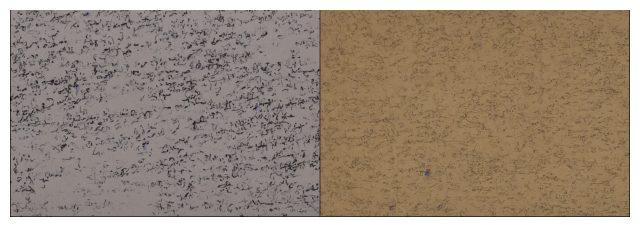
Figure 1. Before domain fine-tuning. The pretrained checkpoint produces music-adjacent texture but not a usable score. It is more accurate to call this the baseline model than an “untrained” model: Stable Diffusion was pretrained, just not on this task.
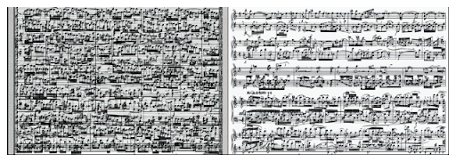
Figure 2. After two fine-tuning epochs. The page geometry, horizontal staves, clef-like shapes, note-like marks, and separation between systems are dramatically clearer.
What improved
Global score structure. The post-training samples contain repeated, parallel staff systems rather than undirected texture. The network learned high-contrast page layout and the local visual vocabulary of music notation.
Symbol density and grouping. Marks are organized around staves and into phrase- or measure-like clusters. The left example is visibly denser than the right, showing that the model varied apparent complexity with instrumentation.
Instrument-specific notation style. Instrument conditioning affected more than the overall appearance of the page. In the qualitative samples, flute and clarinet prompts tended to produce denser, more intricate note sequences, while trumpet and trombone prompts produced comparatively open and less complex passages. These differences reflect how the instruments were represented in the training data and show that the model learned instrument-dependent notational patterns rather than applying one generic musical texture to every prompt.
Key conditioning. The A-minor prompts produced the appropriate natural key signature without sharps or flats. This was a concrete sign that the model was using tonal metadata rather than merely generating an unconditional score page.
Transposing-instrument awareness. The generated scores also reflected that the trumpet is a transposing instrument rather than an instrument in concert pitch. The most common trumpet is tuned to B-flat: a written C sounds as concert B-flat, a major second lower. Therefore, for a B-flat trumpet to sound the same concert C played by a piano, its part must contain a written D (de Ghizé, 2022). The trumpet output adjusted its written notation accordingly instead of treating the trumpet like a piano or another instrument in C. This suggests that the model learned an instrument-specific relationship between written and sounding pitch, not merely a visual association with the word “trumpet.”
Generalization to new descriptions. The project produced coherent sheet-music images from combinations of composer, instrument, and style not encountered during training. Qualitatively, this showed that the model could recombine learned conditions rather than only repeat a single training description.
The limitations that appeared consistently
Line-to-line consistency. The overall generated score structure was coherent, but musical motifs and rhythmic patterns sometimes varied erratically between staves. The issue was intra-page continuity: the model had more difficulty maintaining a compositional idea over the full vertical extent of a page than producing an individual coherent region.
Multiple instruments. Prompts containing more than one instrument sometimes produced roughly six to eleven staff lines without reliably assigning the correct structure to each part. Separate staves could also blend together instead of remaining visually distinct.
The quantitative result—and its limit
This project had a quantitative training objective but mostly qualitative task evaluation.
| Evidence | What was recorded | What it supports |
|---|---|---|
| Data scale | Approximately 10,000 page images | The scope of the experiment |
| Training exposure | 2 epochs; approximately 20,000 example presentations and 10,000 optimizer updates (derived) | How much optimization occurred |
| Noise-prediction loss | MSE, summarized in the poster every 1,000 training samples | Whether the UNet was learning its denoising objective |
| Held-out notation accuracy | Not reported | No numerical claim about valid notes, rhythms, keys, or layout can be made |
| Human or playback evaluation | Not reported | No numerical claim about playability or musical quality can be made |
The source material includes a plotted average training loss but not the underlying numerical series, so exact loss values are not reproduced here. This is a limitation of the archived record, not evidence against the model’s qualitative results. A future run should export the series alongside the plot and add task-specific measurements for key, instrumentation, style, and cross-staff consistency.
The strongest result supported by the surviving artifacts is:
Under the same prompt family, fine-tuning converted unstructured, music-like texture into coherent score-page structure and produced visible differences tied to instrument and key. The remaining qualitative errors were line-to-line consistency and multi-instrument staff layout.
That is a substantial result under limited compute: only two epochs, a roughly 10,000-image subset, and one trainable component.
What the experiment established
The experiment demonstrated four things.
First, the baseline comparison showed that the pretrained checkpoint did not already possess this score-generation behavior. Second, the after-training samples showed a large change in domain structure: staff systems, notation, and page-level organization became clear. Third, controlled prompts showed visible conditioning by instrument and key. Fourth, outputs from new metadata combinations suggested that the model could recombine attributes it had learned from the dataset.
Together, these results support the project’s original hypothesis: a general-purpose latent-diffusion model can be adapted to generate sheet music from natural-language metadata. The two observed failure modes also locate the next research problem precisely—maintaining relationships across distant staff systems and separating several instrumental parts on one page.
A stronger evaluation protocol
A stronger follow-up would turn the observed qualitative behavior into several separate measurements:
- Score structure: measure image quality, staff regularity, symbol clarity, and page layout.
- Can it be parsed? Run optical music recognition and report the proportion of outputs that convert successfully to MusicXML or MIDI.
- Metadata accuracy: check key signature, instrumentation, style, staff count, and instrument-specific range against the prompt.
- Long-range musical consistency: render parsed outputs to audio and use blinded ratings from musicians for motif continuity, rhythmic consistency, style alignment, and playability.
The evaluation split should be grouped by work so neighboring pages cannot leak across train and test. Additional challenge sets could hold out composers, instrument families, keys, and combinations of metadata. Multiple random seeds and the underlying loss values should also be reported.
For prompt conditioning, each metadata field should have its own controlled test. Keep the random seed and all other words fixed, change only the instrument or key, and measure whether the relevant notation changes while unrelated structure remains stable.
Future research
Future work includes more epochs, the 200,000-pair MusicScore split, richer captions, explicit structural constraints, optical music recognition, support for tablature and non-Western notation, and interactive conditioning from a melody or harmonic sketch. Those directions follow directly from the results.
The next version of the same experimental pipeline could be:
full MusicScore-200K corpus
    -> richer page-level captions
    -> aspect-ratio-preserving latent diffusion training
    -> explicit multi-staff layout conditioning
    -> OMR conversion and metric-based evaluation
More data and training would test how far the original architecture scales. Page-level descriptors such as tempo, time signature, form, rhythmic complexity, and staff count would make the conditioning signal more precise. An explicit layout guide could keep multi-instrument staves separate, while an OMR pass would make the outputs searchable, editable, playable, and quantitatively testable.
A consistency objective spanning neighboring crops or staff systems could target the line-to-line problem directly. The broader creative extension from the original project—conditioning on a melody, harmonic sketch, poem, sentence, or emotional description—would then make the system more interactive for musicians and composers.
Discussion
This project demonstrated three levels of progress:
- Domain success: the model learned coherent sheet-music structure instead of generic image texture.
- Conditional success: the output visibly changed in response to instrument, key, style, and composer metadata.
- Compositional consistency: individual regions were coherent, while maintaining motifs across distant staff systems and separating multiple parts remained the next frontier.
The first two appeared clearly in the before-and-after samples. The third explains the two limitations that repeated across the qualitative review.
Fine-tuning produced a dramatic domain shift in only two epochs. More importantly, the conditioning was not limited to the category “sheet music”: the outputs reflected instrument complexity, key signatures, musical style, and new combinations of those descriptors. The project showed how far a carefully constructed image-text dataset and targeted UNet fine-tuning could move a general-purpose model under modest compute.
The central research result is the combination of rapid domain adaptation and controllable generation: a short, targeted fine-tuning run moved a general-purpose model into a specialized notation domain while preserving useful control through natural-language metadata.
Works cited
- de Ghizé, Susan. (2022). “Transposing Instruments.” Steps to Music Theory. Mary and Jeff Bell Library, Texas A&M University–Corpus Christi. Open textbook.
- Ho, Jonathan, Ajay Jain, and Pieter Abbeel. (2020). “Denoising Diffusion Probabilistic Models.” Advances in Neural Information Processing Systems 33. NeurIPS proceedings.
- Ho, Jonathan, and Tim Salimans. (2022). “Classifier-Free Diffusion Guidance.” arXiv:2207.12598.
- Kingma, Diederik P., and Max Welling. (2014). “Auto-Encoding Variational Bayes.” International Conference on Learning Representations. arXiv:1312.6114.
- Lin, Yuheng, Zheqi Dai, and Qiuqiang Kong. (2024). “MusicScore: A Dataset for Music Score Modeling and Generation.” arXiv:2406.11462.
- Loshchilov, Ilya, and Frank Hutter. (2019). “Decoupled Weight Decay Regularization.” International Conference on Learning Representations. OpenReview.
- Radford, Alec, et al. (2021). “Learning Transferable Visual Models from Natural Language Supervision.” Proceedings of the 38th International Conference on Machine Learning, 8748–8763. PMLR.
- Rombach, Robin, Andreas Blattmann, Dominik Lorenz, Patrick Esser, and Björn Ommer. (2022). “High-Resolution Image Synthesis with Latent Diffusion Models.” Proceedings of the IEEE/CVF Conference on Computer Vision and Pattern Recognition, 10684–10695. CVF Open Access.
- Ronneberger, Olaf, Philipp Fischer, and Thomas Brox. (2015). “U-Net: Convolutional Networks for Biomedical Image Segmentation.” Medical Image Computing and Computer-Assisted Intervention, 234–241. arXiv:1505.04597.
- Stable Diffusion v1.5 contributors. (2022). Stable Diffusion v1.5 model card. Hugging Face.